Diffusion Prevalence
The Diffusion Prevalence plot compares the delta-trends of all the statuses allowed by the diffusive model tested.
Each trend line describes the delta of the number of nodes for a given status iteration after iteration.
-
class
ndlib.viz.bokeh.DiffusionPrevalence.DiffusionPrevalence(model, trends)
-
DiffusionPrevalence.__init__(model, iterations)¶ Parameters: - model – The model object
- iterations – The computed simulation iterations
-
DiffusionPrevalence.plot(width, height)¶ Generates the plot
Parameters: - percentile – The percentile for the trend variance area
- width – Image width. Default 500px.
- height – Image height. Default 500px.
Returns: a bokeh figure image
Below is shown an example of Diffusion Prevalence description and visualization for the SIR model.
import networkx as nx
from bokeh.io import show
import ndlib.models.ModelConfig as mc
import ndlib.models.epidemics as ep
from ndlib.viz.bokeh.DiffusionPrevalence import DiffusionPrevalence


# Network topology
g = nx.erdos_renyi_graph(1000, 0.1)

# Model selection
model = ep.SIRModel(g)

# Model Configuration
cfg = mc.Configuration()
cfg.add_model_parameter('beta', 0.001)
cfg.add_model_parameter('gamma', 0.01)
cfg.add_model_parameter("fraction_infected", 16 0.05)
model.set_initial_status(cfg)

# Simulation execution
iterations = model.iteration_bunch(200)
trends = model.build_trends(iterations)

# Visualization
viz = DiffusionPrevalence(model, trends)
p = viz.plot(width=400, height=400)
show(p)
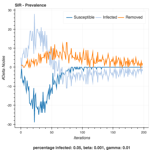
SIR Diffusion Prevalence Example.