Model Multiple Executions
dlib.utils.multi_runs allows the parallel execution of multiple instances of a given model starting from different initial infection conditions.
The initial infected nodes for each instance of the model can be specified either:
- by the “fraction_infected” model parameter, or
- explicitly through a list of
nsets of nodes (wherenis the number of executions required).
In the first scenario “fraction_infected” nodes will be sampled independently for each model execution.
Results of dlib.utils.multi_runs can be feed directly to all the visualization facilities exposed by ndlib.viz.
-
ndlib.utils.multi_runs(model, execution_number, iteration_number, infection_sets, nprocesses)¶ Multiple executions of a given model varying the initial set of infected nodes
Parameters: - model – a configured diffusion model
- execution_number – number of instantiations
- iteration_number – number of iterations per execution
- infection_sets – predefined set of infected nodes sets
- nprocesses – number of processes. Default values cpu number.
Returns: resulting trends for all the executions
Example
Randomly selection of initial infection sets
import networkx as nx
import ndlib.models.ModelConfig as mc
import ndlib.models.epidemics as ep
from ndlib.utils import multi_runs

# Network topology
g = nx.erdos_renyi_graph(1000, 0.1)

# Model selection
model1 = ep.SIRModel(g)

# Model Configuration
config = mc.Configuration()
config.add_model_parameter('beta', 0.001)
config.add_model_parameter('gamma', 0.01)
config.add_model_parameter("fraction_infected", 0.05)
model1.set_initial_status(config)

# Simulation multiple execution
trends = multi_runs(model1, execution_number=10, iteration_number=100, infection_sets=None, nprocesses=4)
Specify initial infection sets
import networkx as nx
import ndlib.models.ModelConfig as mc
import ndlib.models.epidemics as ep
from ndlib.utils import multi_runs

# Network topology
g = nx.erdos_renyi_graph(1000, 0.1)

# Model selection
model1 = ep.SIRModel(g)

# Model Configuration
config = mc.Configuration()
config.add_model_parameter('beta', 0.001)
config.add_model_parameter('gamma', 0.01)
model1.set_initial_status(config)

# Simulation multiple execution
infection_sets = [(1, 2, 3, 4, 5), (3, 23, 22, 54, 2), (98, 2, 12, 26, 3), (4, 6, 9) ]
trends = multi_runs(model1, execution_number=2, iteration_number=100, infection_sets=infection_sets, nprocesses=4)
Plot multiple executions
The ndlib.viz.mpl package offers support for visualization of multiple runs.
In order to visualize the average trend/prevalence along with its inter-percentile range use the following pattern (assuming model1 and trends be the results of the previous code snippet).
from ndlib.viz.mpl.DiffusionTrend import DiffusionTrend
viz = DiffusionTrend(model1, trends)
viz.plot("diffusion.pdf", percentile=90)
where percentile identifies the upper and lower bound (e.g. setting it to 90 implies a range 10-90).
The same pattern can be also applied to comparison plots.
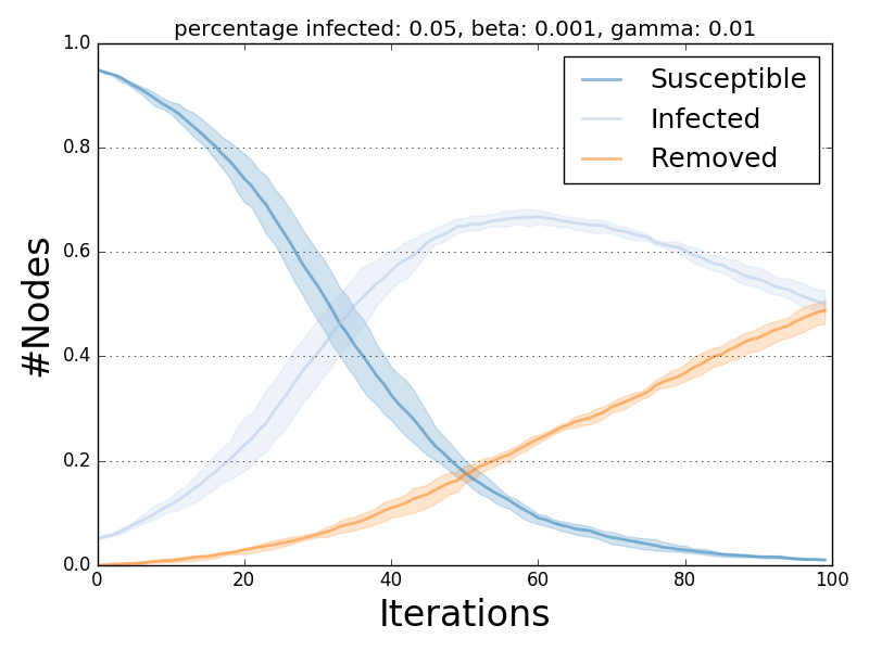
Multiple run visualization.