Model Multiple Executions
dlib.utils.multi_runs allows the parallel execution of multiple instances of a given model starting from different initial infection conditions.
The initial infected nodes for each instance of the model can be specified either:
- by the “fraction_infected” model parameter, or
- explicitly through a list of
nsets of nodes (wherenis the number of executions required).
In the first scenario “fraction_infected” nodes will be sampled independently for each model execution.
Results of dlib.utils.multi_runs can be feed directly to all the visualization facilities exposed by ndlib.viz.
Example
Randomly selection of initial infection sets
import networkx as nx
import ndlib.models.ModelConfig as mc
import ndlib.models.epidemics as ep
from ndlib.utils import multi_runs

# Network topology
g = nx.erdos_renyi_graph(1000, 0.1)

# Model selection
model1 = ep.SIRModel(g)

# Model Configuration
config = mc.Configuration()
config.add_model_parameter('beta', 0.001)
config.add_model_parameter('gamma', 0.01)
config.add_model_parameter("fraction_infected", 0.05)
model1.set_initial_status(config)

# Simulation multiple execution
trends = multi_runs(model1, execution_number=10, iteration_number=100, infection_sets=None, nprocesses=4)
Specify initial infection sets
import networkx as nx
import ndlib.models.ModelConfig as mc
import ndlib.models.epidemics as ep
from ndlib.utils import multi_runs

# Network topology
g = nx.erdos_renyi_graph(1000, 0.1)

# Model selection
model1 = ep.SIRModel(g)

# Model Configuration
config = mc.Configuration()
config.add_model_parameter('beta', 0.001)
config.add_model_parameter('gamma', 0.01)
model1.set_initial_status(config)

# Simulation multiple execution
infection_sets = [(1, 2, 3, 4, 5), (3, 23, 22, 54, 2), (98, 2, 12, 26, 3), (4, 6, 9) ]
trends = multi_runs(model1, execution_number=2, iteration_number=100, infection_sets=infection_sets, nprocesses=4)
Plot multiple executions
The ndlib.viz.mpl package offers support for visualization of multiple runs.
In order to visualize the average trend/prevalence along with its inter-percentile range use the following pattern (assuming model1 and trends be the results of the previous code snippet).
from ndlib.viz.mpl.DiffusionTrend import DiffusionTrend
viz = DiffusionTrend(model1, trends)
viz.plot("diffusion.pdf", percentile=90)
where percentile identifies the upper and lower bound (e.g. setting it to 90 implies a range 10-90).
The same pattern can be also applied to comparison plots.
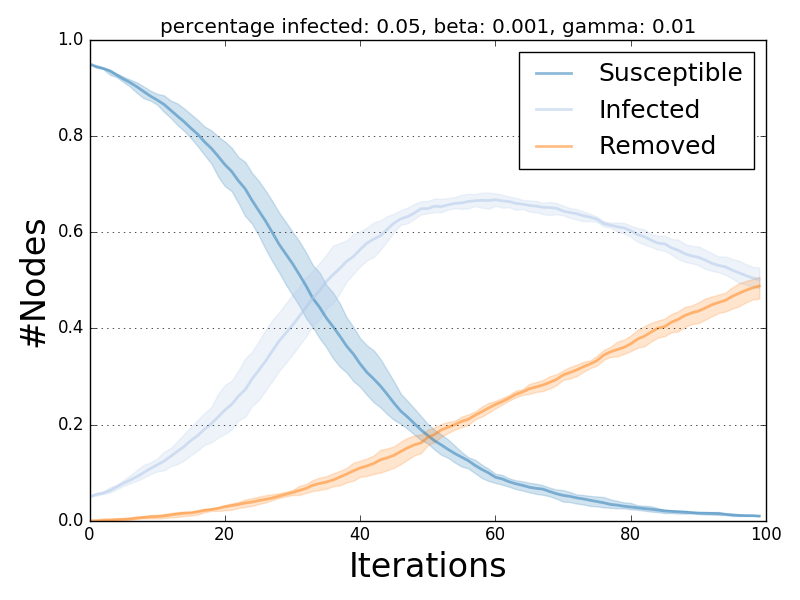
Multiple run visualization.